Multiple Linear Regression

Back to: Machine Learning

Multiple Linear Regression (MLR):

Multiple Linear Regression (MLR) is a statistical technique used to model the relationship between a dependent variable and multiple independent variables. It is an extension of simple linear regression, which deals with just one independent variable.

1. Introduction to Multiple Linear Regression

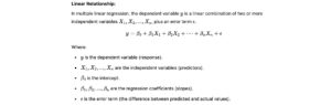
Multiple Linear Regression is used when the dependent variable (also called the response or target variable) depends on two or more independent variables (also known as predictors, features, or explanatory variables).

It is one of the most common techniques in regression analysis, allowing data scientists and statisticians to make predictions or understand relationships in the data.

Real-World Examples:

• Predicting house prices: Using features such as size (square footage), number of rooms, location, etc., to predict the price of a house.
• Sales forecasting: Predicting sales based on advertising budget, marketing spend, and store location.
• Medical predictions: Predicting patient outcomes based on age, weight, lifestyle, and test results.

---

2. The Mathematical Formulation

Goal:

The goal of multiple linear regression is to find the optimal values for β0,β1,…,βn​ that minimize the residual sum of squares (RSS), i.e., the difference between the observed and predicted values of y.

3. Matrix Representation

In multiple linear regression, the equation can be represented in matrix form to simplify the calculations and generalize the solution for more than two predictors.

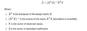
4. Solving for the Coefficients

The optimal coefficients βcan be solved using the Normal Equation, which is derived by minimizing the sum of squared errors (RSS):

 

5. Assumptions in Multiple Linear Regression

For MLR to provide reliable and valid results, the following assumptions should hold:

1. Linearity: The relationship between the dependent and independent variables is linear.
2. Independence: The residuals (errors) are independent of each other.
3. Homoscedasticity: The variance of the residuals is constant across all levels of the independent variables.
4. No multicollinearity: The independent variables are not highly correlated with each other.
5. Normality of Errors: The residuals are normally distributed.

If these assumptions are violated, it can lead to biased coefficients, inefficient estimates, or incorrect conclusions.

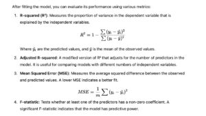
6. Evaluating the Model

7. Assumptions Testing and Diagnostics

1. Residual Plots: Plot residuals to check for homoscedasticity. If the residuals fan out or form patterns, the model may not fit well.
2. VIF (Variance Inflation Factor): Checks for multicollinearity. If the VIF is greater than 10 for a variable, it indicates a high correlation with other variables.
3. QQ Plot: Check the normality of residuals. If the residuals deviate significantly from the diagonal, the normality assumption is violated.

Step-by-Step Calculation with Simple Data:

Let’s consider a simple example with two independent variables (features) and one dependent variable.

Data:

We have the following sample data:

Where:

• X1 and X2 are the independent variables.
• y is the dependent variable.

Step 1: Construct the Design Matrix $X$

To include the intercept, we add a column of ones to the matrix X.

Here, the first column is the ones for the intercept term, and the second and third columns are the values of X1 and X2.

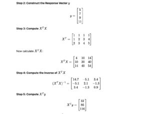
Step 6: Calculate the Coefficients β

Interpretation:

The coefficients are:

• β0=2 (intercept),
• β1=1 (coefficient for X1),
• β2=1(coefficient for X2).

Thus, the model is:

y=2+1.X1+1.X2​

This means for every unit increase in X1or X2, the dependent variable y increases by 1.

​