Ensembling Algorithm

Back to: Machine Learning

Ensembling Techniques in Machine Learning

Ensembling techniques are powerful methods in machine learning that combine the predictions of multiple models to improve the overall performance of a machine learning system. By aggregating the results from various models, ensembling can enhance the accuracy, reduce the risk of overfitting, and increase the robustness of predictions compared to individual models.

Key Benefits of Ensembling:

1. Reduces Overfitting: Ensembling combines the predictions of multiple models, smoothing out individual model errors and making the system less likely to overfit to noise in the training data.
2. Improves Accuracy: By leveraging the strengths of different models, ensembling can improve the overall accuracy, especially in cases where individual models perform differently on various subsets of data.
3. Enhances Robustness: Aggregating diverse models makes the overall prediction more stable and reliable, reducing the impact of model-specific errors or biases.

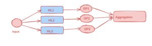
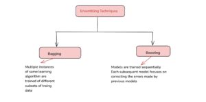
Ensembling algorithms can work in two ways:

1. Same Model, Different Data (Bagging) – Multiple instances of the same model are trained on different subsets of the data, and their predictions are combined. Example: Random Forest.
2. Same Model, Sequential Learning (Boosting) – Models are trained one after another, where each new model corrects the errors of the previous one. Example: AdaBoost, XGBoost.

Bagging (Bootstrap Aggregating) in Machine Learning

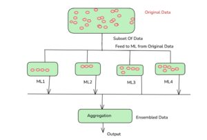
Bagging is a type of ensemble technique in which multiple models of the same type are trained on different subsets of the data. These subsets are created using bootstrapping, which means sampling the data with replacement. After the models are trained, their predictions are combined by averaging (for regression) or majority voting (for classification) to make the final prediction.

The goal of bagging is to reduce variance and prevent overfitting, improving the model’s generalization ability.

How Bagging Works:

1. Generate Subsets: The original dataset is randomly sampled with replacement to create multiple training subsets (these may overlap).
2. Train Models: A model is trained on each subset of the data.
3. Aggregate Predictions: The final prediction is made by combining the predictions from all models. For classification, the most frequent class (majority vote) is chosen, and for regression, the average of all predictions is taken.

Sample Tabular Data:

Imagine we have a small dataset with 5 data points and a target class variable (for classification):

Feature 1	Feature 2	Target (Class)
1	2	A
2	3	B
3	4	A
4	5	B
5	6	A

Steps of Bagging:

1. Create Bootstrapped Subsets:
   Randomly sample data points from the original dataset with replacement. Each subset may contain repeated data points.
   • Subset 1: [(1,2), (2,3), (3,4), (5,6), (1,2)]
   • Subset 2: [(4,5), (5,6), (3,4), (2,3), (2,3)]
   • Subset 3: [(1,2), (4,5), (3,4), (5,6), (3,4)]
2. Train Models on Subsets:
   Train a decision tree (or any model) on each subset:
   • Model 1 (trained on Subset 1)
   • Model 2 (trained on Subset 2)
   • Model 3 (trained on Subset 3)
3. Make Predictions:
   Suppose we want to predict the class for the new data point (Feature 1 = 3, Feature 2 = 4). The models give the following predictions:
   • Model 1: A
   • Model 2: B
   • Model 3: A
4. Aggregate Predictions:
   For classification, the final prediction is made by taking a majority vote:
   • A: 2 votes
   • B: 1 vote
   • Final Prediction: A (since A has the majority vote).

Advantages of Bagging:

• Reduces Overfitting: By training models on different subsets of data, bagging reduces the risk of overfitting, especially for high-variance models like decision trees.
• Improves Accuracy: Multiple models trained on different data points lead to more reliable predictions.
• Parallelization: Since each model is trained independently, bagging can be easily parallelized for faster training.

Bootstrapping in Machine Learning

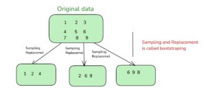
Bootstrapping is a statistical technique where multiple samples are drawn from the original dataset with replacement. This means that some data points might appear multiple times in the sampled data, while others might not appear at all. This is particularly useful when you want to create multiple datasets for training different models (such as in Bagging).

How Bootstrapping Works:

1. Sample with Replacement: From the original dataset, random samples are taken with replacement, meaning that each point can be selected multiple times.
2. Fraction of the Data: Typically, a bootstrapped sample contains about the same number of data points as the original dataset, though it may have some duplicate points and others may be missing.
3. Out-of-Bag (OOB) Samples: The points that are not selected in a given bootstrap sample are called Out-of-Bag (OOB) samples. These OOB samples can be used for validation or to estimate model performance without needing an extra validation dataset.

Important Terms:

• Bagging Fraction: The fraction of the original dataset used in each bootstrap sample (usually, it’s 1.0, meaning each bootstrap sample is the same size as the original dataset).
• OOB Fraction: The fraction of the original dataset that is not selected for a particular bootstrap sample. Typically, about 1/3 of the original dataset will be OOB in each bootstrapped sample (since 2/3 of the data is usually selected).

Sample Tabular Data:

Let’s take a small dataset with 5 data points:

Feature 1	Feature 2	Target (Class)
1	2	A
2	3	B
3	4	A
4	5	B
5	6	A

Bootstrapping Example:

Step 1: Original Dataset

• The dataset has 5 data points.

Step 2: Create Bootstrapped Samples

Let’s generate 3 bootstrapped samples, each containing 5 points (same size as the original dataset). Since we are sampling with replacement, some points might be repeated, and some might be missing.

Bootstrapped Sample 1:

Feature 1	Feature 2	Target (Class)
1	2	A
1	2	A
3	4	A
4	5	B
2	3	B

Bootstrapped Sample 2:

Feature 1	Feature 2	Target (Class)
5	6	A
3	4	A
4	5	B
5	6	A
1	2	A

Bootstrapped Sample 3:

Feature 1	Feature 2	Target (Class)
3	4	A
2	3	B
1	2	A
5	6	A
4	5	B

Step 3: Out-of-Bag (OOB) Samples

The data points that are not included in a given bootstrap sample are called Out-of-Bag samples.

Out-of-Bag for Sample 1:

• The OOB samples are: (2,3), (4,5), (5,6). These samples were not selected in Sample 1 and can be used for validation.

Out-of-Bag for Sample 2:

• The OOB samples are: (2,3), (4,5). These samples were not selected in Sample 2 and can be used for validation.

Out-of-Bag for Sample 3:

• The OOB samples are: (2,3), (5,6). These samples were not selected in Sample 3 and can be used for validation.

Step 4: Summary of OOB and Bagging Fraction

• Bagging Fraction: The bagging fraction is the fraction of the original dataset used in each bootstrapped sample. In this case, it is 1.0 (since each bootstrapped sample has the same number of points as the original dataset).
• OOB Fraction: On average, about 1/3 of the data points are OOB. For example, in Sample 1, the OOB points are (2,3), (4,5), (5,6), which constitute 3 out of 5 data points or 60% of the original dataset.

Visualizing the Process:

Bootstrapped Sample	OOB Sample
(1,2), (1,2), (3,4), (4,5), (2,3)	(5,6)
(5,6), (3,4), (4,5), (5,6), (1,2)	(2,3)
(3,4), (2,3), (1,2), (5,6), (4,5)	(2,3)

Advantages of Bootstrapping:

1. Reduces Bias: By using different samples of data, bootstrapping reduces the risk of bias in the model.
2. Improves Stability: Bootstrapping provides multiple models trained on different data subsets, helping to create a more stable and reliable final prediction.
3. OOB Validation: Bootstrapping automatically provides a validation set for each model (OOB samples) without needing to create a separate validation dataset.