Back to: Machine Learning
Introduction to Classification in Machine Learning
In machine learning, classification is a fundamental type of supervised learning where the goal is to assign an input to a specific category or label based on its characteristics. It’s a powerful tool used in various real-world applications, from spam detection to disease diagnosis and image recognition.
What is Classification?
At its core, classification involves taking an input (which could be anything like an email, medical record, or image) and predicting a label or category for it. The input is represented by a set of features, and the output is a class or category. The machine learning model learns the relationship between these features and their associated labels from a labeled dataset (a dataset where the correct label for each input is known).
How Classification Works
In a classification problem, you are given a dataset that consists of pairs (X1,Y1),(X2,Y2),…,(Xn,Yn) where:
- Xi represents the features or input data.
- Yi is the class label or output that corresponds to each input.
The goal is to learn a model, f(x) that can predict the class yfor a new, unseen instance x.
Types of Classification Problems
Classification problems can be divided into different types, depending on the nature of the output classes:
- Binary Classification:
This type involves only two possible classes. For instance, in spam detection, an email is classified as either spam or not spam. Another example could be predicting whether a customer will buy or not buy a product. - Multiclass Classification:
Here, the output consists of more than two classes. For example, in digit recognition, the task might be to classify an image as one of the digits (0-9). It’s not just about saying yes or no, but assigning one of several possible labels. - Multilabel Classification:
In multilabel classification, an instance can belong to more than one class simultaneously. For example, a movie can be classified as both a comedy and an action film at the same time. Each instance can have multiple labels that apply.
Understanding Input Interpretation in Classification: A Simple Guide
When we build machine learning models to classify data, the way we handle the input data is very important. Different types of data (features) need different ways of being processed. Let’s break down the most common types of features you’ll encounter.
1. Numerical Features: Numbers That Measure Something
Numerical features are data that represent quantities or measurements. These are numbers that can vary widely, like:
- Age
- Salary
- Height
- Temperature
These features are straightforward because the model can directly use these numbers. However, sometimes we may need to adjust the numbers to make them easier for the model to understand, like by scaling them to similar ranges.
2. Categorical Features: Grouping Things into Categories
Categorical features are data that represent different groups or categories. For example:
- Gender
- Color
- Marital status
Since these features are not numbers, we need to convert them into numbers before the model can use them. This is done by techniques like one-hot encoding, which turns each category into a separate column with 1s and 0s.
3. Textual Features: Turning Words Into Numbers
Text data, like articles, reviews, or messages, can also be used as input. But since computers can’t directly understand words, we need to turn them into numbers. We do this using methods like:
- Bag of Words (turns text into a list of word counts)
- TF-IDF (gives more importance to unique words)
- Word Embeddings (turns words into numbers that capture their meaning)
This allows the model to understand the content of the text and use it to make predictions.
4. Image Features: Working With Pixels
Images are made up of pixels, and each pixel has a color value. To use images in machine learning, we need to convert the pixels into numbers. For simple tasks, we might just use the raw pixel values, but for more complex tasks, we use special models like Convolutional Neural Networks (CNNs) to automatically find patterns in the image.
Handling categorical features – categorical features cannot be directly used by most machine learning algorithms since they except numerical inputs . therefore categorical inputs must be encoded into numerical features.
A Beginner’s Guide to Categorical Data and Encoding Techniques
When working with machine learning models, data preprocessing is a crucial step that ensures the data is suitable for analysis. One common type of data we encounter is categorical data, which can be classified into two main types: ordinal and nominal. Understanding these types and their encoding methods is vital to building effective models.
Types of Categorical Data
1. Ordinal Data
Ordinal data represents categories with a meaningful order or ranking. For example:
- Levels of confidence:
- Less confident
- Slightly confident
- Very confident
Here, the sequence carries significance, as “Very confident” ranks higher than “Less confident.”
2. Nominal Data
Nominal data represents categories without any inherent order. For example:
- Colors:
- Red
- Green
- Blue
In this case, the categories are distinct but unordered.
Encoding Categorical Data
Machine learning algorithms work with numerical input, so categorical data must be converted into numerical formats. The two most common encoding methods are label encoding and one-hot encoding.
Label Encoding
This technique assigns a unique numerical value to each category.
Example:
- Colors:
- Red = 0
- Green = 1
- Blue = 2
- Levels of confidence:
- Less confident = 0
- Slightly confident = 1
- Very confident = 2
Pros:
- Simple and efficient.
- Works well with ordinal data, where the numerical values represent meaningful rankings.
Cons:
- Not ideal for nominal data. The model may misinterpret the numerical values as ordinal relationships, introducing bias.
One-Hot Encoding
This method creates a new binary feature for each category, assigning 1 if the category is present and 0 otherwise.
Example:
For colors (Red, Green, Blue):

Pros:
- Avoids the pitfalls of ordinal relationships for nominal data.
- Provides clear separation of categories.
Cons:
- Increases dimensionality, especially for datasets with many categories. This can lead to higher computational costs and model complexity.
Choosing the Right Encoding Technique
- Use label encoding for ordinal data, where the order matters.
- Use one-hot encoding for nominal data to eliminate unintended ordinal relationships.
Example Dataset: Age, Gender, Subscription, and Purchase
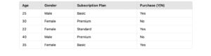
Identifying Nominal and Ordinal Data
- Age:
- Type: Continuous numerical data (neither nominal nor ordinal in this case).
- Gender:
- Type: Nominal
- Categories like “Male” and “Female” have no inherent order.
- Subscription Plan:
- Type: Ordinal
- Categories (Basic, Standard, Premium) can be ranked based on the level of service provided.
- Purchase (Y/N):
- Type: Binary categorical data (Nominal).
Data Encoding
Label Encoding for Subscription Plan (Ordinal Data):

One-Hot Encoding for Gender (Nominal Data):

Transformed Dataset

Handling Numerical Data in Machine Learning: Best Practices
Numerical data forms the backbone of many machine learning models, as most algorithms work natively with numerical inputs.
However, to ensure accurate predictions and model efficiency, proper preprocessing of numerical features is essential. This blog outlines three critical aspects of handling numerical data: feature scaling, outlier management, and dealing with missing data.
1. Feature Scaling
Numerical features often vary in scale, which can impact the performance of models sensitive to these differences (e.g., gradient descent-based algorithms like linear regression, SVM, and neural networks). Feature scaling transforms the data to ensure all features contribute equally during model training.
Common Scaling Techniques
- Min-Max Scaling
Rescales values to a fixed range, typically [0, 1].Formula:- Pros: Preserves the data’s original distribution.
- Cons: Sensitive to outliers.
- Standardization
Centers the data around zero with a standard deviation of one.Formula:where μ is the mean and σ is the standard deviation.- Pros: Robust to outliers; suitable for algorithms assuming Gaussian distributions.
- Cons: May not fit well if data isn’t normally distributed.


2. Handling Outliers
Outliers can skew the results of machine learning models, especially those relying on distance metrics or sensitive to extreme values. Proper handling is crucial for maintaining model stability.
Common Techniques
- Clipping
- Restricts feature values to a predefined range.
- Example: Capping values above the 95th percentile or below the 5th percentile.
Pros: Prevents extreme values from dominating the analysis.
Cons: May result in loss of information about true extremes. - Log Transformation
- Compresses the scale of large numbers by applying the logarithmic function.
- Example: Transforming salaries or population counts to reduce variance.
Pros: Reduces skewness, making the data more normally distributed.
Cons: Ineffective for data with zero or negative values (requires adjustments).
3. Dealing with Missing Data
Missing data is a common issue that can degrade model performance or introduce bias. Choosing the right approach depends on the extent and nature of the missing data.
Approaches
- Removal
- Row Removal: Excludes rows with missing values.
- Column Removal: Drops features with significant missing values.
Pros: Simple and quick to implement.
Cons: Can lead to significant data loss, reducing the model’s ability to generalize. - Imputation
- Fills missing values with estimates such as:
- Mean: Suitable for symmetrical distributions.
- Median: Ideal for skewed data.
- Mode: Best for categorical-like numerical features.
Pros: Retains all data points and reduces loss of information.
Cons: Introduces estimation bias if not done carefully. - Fills missing values with estimates such as:
Understanding Output Interpretation in Classification Models
Classification models aim to categorize data into predefined classes. However, the way these models present their predictions varies based on the algorithm and its configuration. This blog explores the different forms of outputs produced by classification models, the role of thresholding in decision-making, and the functions that enable probability estimation.
1. Class Probabilities
Many classification algorithms, such as logistic regression and neural networks, provide output in the form of class probabilities. This output represents a probability distribution over the possible classes, indicating the likelihood of the input belonging to each class.
Example: Email Classification
- Model Output:
- Spam: 0.73
- Not Spam: 0.27
- Interpretation: The model predicts a 73% chance that the email is spam and a 27% chance it is not.
This format allows flexibility, as thresholds can be applied to determine the final class label.
2. Class Labels
Other classification algorithms, such as decision trees and k-nearest neighbors (KNN), directly assign an output to one of the predefined classes. These models skip probability estimation and provide discrete class labels based on their decision-making rules.
Example: Image Classification
- Model Output: Cat
- Interpretation: The model directly identifies the input image as a “Cat” without providing confidence scores.
While simpler to interpret, this format lacks the nuanced insights offered by probabilities.
3. Thresholding
For models that output probabilities, a threshold is applied to convert probabilities into class labels. By default, thresholds like 0.5 are used in binary classification, but they can be adjusted to balance precision and recall based on the specific application.
Example: Medical Diagnosis (Binary Classification)
- Probability Output:
- Disease: 0.6
- No Disease: 0.4
- Threshold: 0.5
- Decision: Since 0.6 > 0.5, the model classifies the instance as “Disease.”
Adjusting the threshold:
- Lower Threshold: Increases sensitivity (recall), reducing false negatives.
- Higher Threshold: Increases precision, reducing false positives.
4. Activation Functions for Probability Estimation
Modern classification models often rely on activation functions to produce normalized probabilities for their outputs.
Softmax Function (Multiclass Classification)
The softmax function is used when the output involves multiple classes. It converts raw model outputs (logits) into a probability distribution, ensuring the probabilities sum to 1.
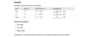
Example:
- Model Output:
- Dog: 0.7
- Cat: 0.2
- Rabbit: 0.1
- Interpretation: The model is most confident that the input is a “Dog.”
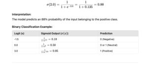
Sigmoid Function (Binary Classification)
The sigmoid function maps raw outputs to probabilities between 0 and 1, typically for binary classification tasks.
Formula:
Example:
- Model Output: 0.8
- Interpretation: The instance has an 80% likelihood of belonging to the positive class.
Softmax Function: Understanding the Key to Multiclass Classification
The softmax function is a mathematical function commonly used in machine learning for multiclass classification problems.
It transforms raw model outputs (known as logits) into probabilities, which represent the likelihood of each class. The probabilities generated by softmax are normalized, meaning they sum up to 1, making them interpretable as confidence scores.
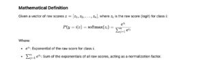
How It Works
- Exponentiation:
The logits (raw scores) are converted to positive numbers by taking the exponential, which amplifies larger logits and diminishes smaller ones. - Normalization:
Each exponential value is divided by the sum of all exponentials, ensuring that the resulting probabilities sum up to 1.
Sigmoid Function: A Fundamental Tool for Binary Classification
The sigmoid function is a widely used activation function in machine learning, especially for binary classification tasks. It transforms raw model outputs (logits) into probabilities between 0 and 1, making it ideal for tasks where the goal is to predict the likelihood of a single class.
Mathematical Definition
The sigmoid function σ(x) is defined as:

Where:
- X: Input value (logit) from the model.
- e: Euler’s number, approximately 2.718.
The function maps any real number X to a value between 0 and 1.
How It Works
- Range Compression:
- The exponential term ensures that the output of the sigmoid function stays within the range (0, 1).
- Positive X: Output approaches 1 as X increases.
- Negative X: Output approaches 0 as X decreases.
- Probabilistic Output:
- The sigmoid function interprets the output as the probability of belonging to the positive class.
Key Properties
- Output Range:
- Always between 0 and 1, making it suitable for representing probabilities.
- S-Shaped Curve:
- Smooth and continuous, making it differentiable for optimization purposes.
- Symmetry:
- The function is symmetric around x=0.
- Interpretation:
- Outputs greater than 0.5 are typically classified as positive class (1).
- Outputs less than 0.5 are classified as negative class (0).
Example
Raw Logit Outputs:
Suppose a logistic regression model outputs the following logits:
- x=2.0
Sigmoid Calculation:
Applications of the Sigmoid Function
- Binary Classification:
- Used in algorithms like logistic regression and the output layer of neural networks for binary problems.
- Probability Estimation:
- Converts raw model outputs into interpretable probabilities.
- Neural Network Activation:
- Historically used as an activation function in hidden layers (though ReLU is more common now).
Advantages of Sigmoid
- Smooth Differentiability:
- The sigmoid function is differentiable, making it compatible with gradient-based optimization algorithms.
- Probabilistic Interpretation:
- Outputs are naturally scaled to represent probabilities.
- Simple and Intuitive:
- The S-shaped curve is easy to understand and implement.
Limitations of Sigmoid
- Vanishing Gradient Problem:
- For very large or very small inputs, the gradient (derivative) approaches zero, slowing down model training.
- Not Zero-Centered:
- Outputs are always positive, which can slow down optimization when used in hidden layers.
- Limited Use in Multiclass Problems:
- For multiclass classification, the softmax function is preferred.