Regularization,Lasso & Ridge Regression

Regularization, Lasso, and Ridge Regression: A Guide to Controlling Overfitting

Introduction to Regularization

Regularization is a powerful technique to improve the performance of machine learning models, especially regression models like multiple linear regression.

Its primary goal is to prevent overfitting—a phenomenon where the model becomes too complex and starts capturing not only the underlying data patterns but also the noise, resulting in poor performance on unseen data.

How Regularization Works

In regression models, overfitting often occurs when the coefficients of the features become excessively large, allowing the model to fit the training data too well. Regularization counters this by adding a penalty term to the loss function. This penalty discourages large coefficients, making the model:

Simpler: By reducing the magnitude of coefficients, the model focuses on the most relevant features.
Generalizable: A less complex model performs better on unseen data.

Mathematically, the modified loss function becomes:

Loss Function=Sum Square Error+Penalty Term

Types of Regularization: Lasso and Ridge Regression

Lasso Regression (L1 Regularization)
- Adds the L1 norm of the coefficients as a penalty:
- Encourages sparsity in the model by shrinking some coefficients to exactly zero, effectively performing feature selection.
- Use Case: When only a subset of features is expected to contribute significantly to the target variable.
Ridge Regression (L2 Regularization)
- Adds the L2 norm of the coefficients as a penalty:
- Shrinks coefficients towards zero but doesn’t make them exactly zero.
- Use Case: When all features are expected to contribute but need to be regularized to avoid overfitting.
Elastic Net (Combination of L1 and L2 Regularization)
- Balances feature selection (L1) and coefficient shrinkage (L2).

Here’s a step-by-step guide with examples and manual calculations for Lasso Regression, Ridge Regression, and Elastic Net

Problem Statement

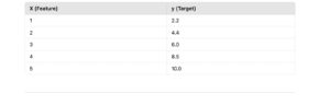
You have the following dataset with two features () and a target variable ():

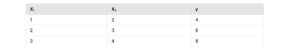
We aim to fit a regression model:

$β_{0} + β_{1} X_{1} + β_{2} X_{2}$

Ordinary Least Squares (OLS) Regression

OLS minimizes the Residual Sum of Squares (RSS):

Calculations:

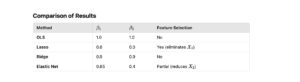
After solving (manually or via matrix multiplication), the coefficients are: $β_{0} = 2, β_{1} = 1, β_{2} = 1$

The resulting model is:

However, OLS does not handle overfitting, so we apply regularization techniques to improve the model.

Lasso Regression (L1 Regularization)

Objective Function:

$Lasso Loss = RSS + λ \sum ∣ β_{i} ∣$

Explanation:

Adds a penalty proportional to the absolute values of coefficients ().
Can shrink some coefficients to exactly zero, effectively selecting features.

Example:

Let :

$Lasso Loss = RSS + 1 \cdot (∣ β_{1} ∣ + ∣ β_{2} ∣)$

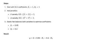
Steps:

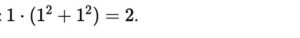
Start with OLS coefficients: .
Add the penalty: .
Lasso reduces coefficients to minimize the total loss:
- (Lasso shrinks this coefficient to zero).

Result:

$y = 2 + 0.8 \cdot X_{1}$

Interpretation: Lasso eliminates $X_{2}$ from the model, indicating it is not essential.

Ridge Regression (L2 Regularization)

Objective Function:

Explanation:

Adds a penalty proportional to the square of coefficients ( $β_{i 2}$ ).
Shrinks coefficients close to zero but does not eliminate them.

Steps:

Start with OLS coefficients: .
Add the penalty:
Ridge adjusts coefficients to reduce the total loss:

Result:

Interpretation: Ridge keeps all features but reduces their influence.

Elastic Net (Combination of L1 and L2 Regularization)

Objective Function:

Elastic Net Loss=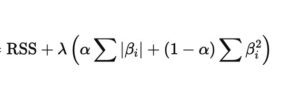

Explanation:

Combines Lasso (L1) and Ridge (L2) penalties.
Balances between shrinking coefficients and feature selection.

Example:

Let and :

Elastic Net Loss=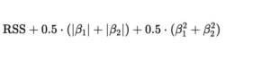

Interpretation: Elastic Net selects important features (like Lasso) while retaining some impact from others (like Ridge).

Overfitting vs. Underfitting

In machine learning, overfitting and underfitting are two critical problems that arise during model training:

1. Overfitting

Definition:
Overfitting occurs when a model learns not only the patterns in the training data but also the noise. This leads to excellent performance on the training data but poor generalization to new, unseen data.
Characteristics:
- High accuracy on the training set.
- Poor performance on the test/validation set.
- The model is too complex for the given data.

2. Underfitting

Definition:
Underfitting occurs when a model is too simple to capture the underlying patterns in the data. It fails to perform well on both training and test datasets.
Characteristics:
- Low accuracy on the training set.
- Poor performance on the test/validation set.
- The model lacks the capacity to learn the relationships in the data.

Example with Images

We’ll illustrate overfitting, underfitting, and a well-fitted model using a regression task:

Dataset:

A simple dataset with a non-linear trend:

Underfitting Example

Model: A linear regression model (too simple).

The model assumes a straight-line relationship, failing to capture the non-linear trend in the data.

Visualization:
Imagine a straight line barely touching the data points.

Overfitting Example

Model: A high-degree polynomial regression model (too complex).

The model fits the training data perfectly by creating a wavy curve, capturing even minor fluctuations (noise).
On new data, the model performs poorly.

Visualization:
A wavy line passing exactly through all the data points but behaving erratically for unseen values.

Well-Fitted Model

Model: A moderately complex polynomial regression (e.g., quadratic).

The model captures the trend of the data without overfitting the noise.
It generalizes well to new data.

Visualization:
A smooth curve closely following the data trend.

Creating the Visuals

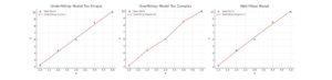
Visual Explanation

Underfitting (Left Plot):
- The red line is too simple (a straight line) and does not capture the data’s trend.
- It represents a model that cannot explain the relationship between $X$ and $y$ .
Overfitting (Middle Plot):
- The red line fits all the data points perfectly but is overly wavy.
- It captures the noise in the data, leading to poor generalization to new data.
Well-Fitted Model (Right Plot):
- The red line is a smooth curve that follows the data trend without being overly complex.
- It strikes a balance between bias and variance, making it a good model for generalization.

Regularization, Lasso, and Ridge Regression: A Guide to Controlling Overfitting

Introduction to Regularization

How Regularization Works

Loss Function=Sum Square Error+Penalty Term

Types of Regularization: Lasso and Ridge Regression

Here’s a step-by-step guide with examples and manual calculations for Lasso Regression, Ridge Regression, and Elastic Net

Problem Statement

y=β0​+β1​X1​+β2​X2

Ordinary Least Squares (OLS) Regression

Calculations:

y=2+1⋅X1​+1⋅X2​

Lasso Regression (L1 Regularization)

Lasso Loss=RSS+λ∑∣βi​∣

Example:

​

Ridge Regression (L2 Regularization)

y=2+0.9⋅X1+0.9⋅X​

Elastic Net (Combination of L1 and L2 Regularization)

Example:

Overfitting vs. Underfitting

1. Overfitting

2. Underfitting

Example with Images

Dataset:

Underfitting Example

Overfitting Example

Well-Fitted Model

Creating the Visuals

Visual Explanation

Leave a Reply Cancel reply

$β_{0} + β_{1} X_{1} + β_{2} X_{2}$

$Lasso Loss = RSS + λ \sum ∣ β_{i} ∣$