Back to: Machine Learning
Introduction: Understanding Gradient Descent for MLR
In the world of machine learning, one of the most widely used optimization techniques is Gradient Descent.
When applied to Multiple Linear Regression (MLR), it helps us find the optimal coefficients (weights) that minimize the cost function (usually Mean Squared Error, or MSE).
This optimization technique is crucial for fitting models to data when an analytical solution (like the Normal Equation) is computationally expensive or infeasible for large datasets.
In this blog, we’ll dive into how gradient descent works in the context of MLR, explaining the underlying math, the iterative nature of the algorithm, and how to implement it efficiently using Python.
What is Multiple Linear Regression (MLR)?
Multiple Linear Regression is an extension of simple linear regression, where the goal is to model the relationship between a dependent variable y and multiple independent variables X1,X2,…,Xn.
The general equation for MLR is: y=β0+β1X1+β2X2+⋯+βnXn+ϵ
Where:
- y is the dependent variable.
- X1,X2,…,Xn are the independent variables (features).
- is the intercept (bias term).
- β1,β2,…, are the regression coefficients (weights).
- ϵ(epsilon) is the error term.
The goal of regression is to find the optimal values for the coefficients β0,β1,…,βn that minimize the cost function (typically Mean Squared Error or MSE).
Understanding Gradient Descent
Gradient Descent is an optimization algorithm used to minimize the cost function in regression problems. It is an iterative method that adjusts the coefficients based on the gradient (or derivative) of the cost function.
The basic idea is to update the coefficients in the direction opposite to the gradient of the cost function. This means we move downhill, minimizing the cost function until we reach the optimal point (local minimum).
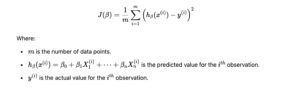
Cost Function (MSE):
For Multiple Linear Regression, the Mean Squared Error (MSE) is commonly used as the cost function:
Gradient Descent Update Rule:
In gradient descent, we update the coefficients iteratively based on the partial derivative of the cost function with respect to each coefficient:

Where:
- α(alpha) is the learning rate (a hyperparameter that determines the step size).

Steps in Gradient Descent for MLR
- Initialize the Coefficients: Start with initial guesses for β0,β1,…,βn. These can be set to zero or small random values.
- Calculate the Hypothesis: For each data point, compute the predicted value hβ(x) using the current values of the coefficients.
- Compute the Cost Function: Calculate the MSE (or another cost function) to evaluate how well the current coefficients fit the data.
- Update the Coefficients: Use the gradient descent update rule to adjust the coefficients in the direction of the negative gradient.
- Repeat: Repeat steps 2-4 for a fixed number of iterations or until the change in the cost function is smaller than a set threshold.
- Convergence: The algorithm converges when the coefficients no longer change significantly, indicating that the minimum cost has been reached.
Python Implementation: Gradient Descent for MLR
Here’s a simple Python code to implement Gradient Descent for Multiple Linear Regression using NumPy:
- import numpy as np
- # Sample data (X1, X2 as features, y as target)
X = np.array([[1, 1, 2], [1, 2, 3], [1, 3, 4], [1, 4, 5]]) # Adding 1 for intercept term
y = np.array([5, 7, 9, 11]) # Target values - # Hyperparameters
alpha = 0.01 # Learning rate
iterations = 1000 # Number of iterations
m = len(y) # Number of data points - # Initialize coefficients (beta values) to zero
beta = np.zeros(X.shape[1]) - # Gradient Descent algorithm
for i in range(iterations):
# Compute the hypothesis (predictions)
predictions = np.dot(X, beta)# Compute the error (difference between predicted and actual values)
error = predictions – y# Compute the gradient
gradient = (1/m) * np.dot(X.T, error)# Update the coefficients using the gradient descent rule
beta -= alpha * gradient - # Output the final coefficients
print(“Optimized coefficients:”, beta)
Advantages and Limitations of Gradient Descent for MLR
Advantages:
- Scalability: Gradient descent can handle large datasets efficiently, especially when the number of features is large.
- Flexibility: It can be used in a variety of optimization problems, not just for MLR.
- Memory Efficiency: Unlike the Normal Equation, gradient descent doesn’t require the computation of the matrix inverse, making it more memory-efficient for very large datasets.
Limitations:
- Choice of Learning Rate: The learning rate α\alpha is critical. If it’s too small, convergence will be slow; if it’s too large, the algorithm may overshoot the minimum.
- Local Minima: For some cost functions, gradient descent may converge to local minima instead of the global minimum, though this is less of an issue with convex functions like MSE.
- Convergence Speed: Gradient descent may require many iterations to converge, especially for complex models with many features.
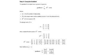
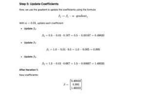
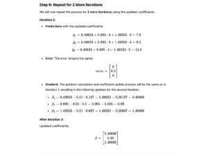
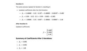
Let’s walk through the process of calculating Gradient Descent for Multiple Linear Regression manually for 3 iterations with a sample dataset. This will help you understand how the coefficients are updated step by step.
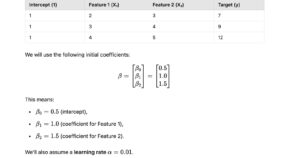
Step 1: Sample Data
Consider the following dataset with 3 data points and 2 features (excluding the intercept term):
Step 2: Prediction Calculation
The formula for predictions in multiple linear regression is:
y^=β0+β1⋅X1+β2⋅X2
Using the initial coefficients, we calculate the predictions for each data point:
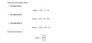
- For Data Point 1: